Creating a large-scale interactive force-directed graph

In this blog post, we will explore how to create a force-directed graph using the latest versions of two libraries: PIXI.js v7 and D3 v7. By combining the rendering capabilities of PIXI.js with the force simulation abilities of D3.js, particularly the d3-force module, you can build performant force-directed graphs for your web applications.

PIXI.js leverages hardware acceleration through WebGL, making it well-suited for rendering data visualizations that involve a significant amount of data points, interactivity or real-time updates. Similar to D3.js, PIXI.js gives you great control over the graphical elements to create custom visual effects and styles.

This is the first article of a three-part series delving deep into the creation of a suite of features or functionality associated with interactive and filterable graphs not meant just to present connections, but also to hopefully encourage data exploration as a graph analytical tool.

Readers should have some experience with D3.js and the d3-force module. Basic knowledge of PIXI.js is useful but not required. I will start off with the webpage setup and data processing work.

Getting Started

Before diving into the implementation, let’s set up a basic project structure. You can create a directory for your project and include the necessary libraries. Create an index.html file containing a DIV element to render the graph in.

Initialize your project and install PIXI.js and D3.js using npm.

npm init
npm install pixi.js pixi-viewport d3

Create a Javascript file to write code to generate the force-directed graph. Import the installed modules.

import * as PIXI from "pixi.js";
import { Viewport } from "pixi-viewport";
import * as d3 from "d3";

Data preparation

Ensure you have a separate dataset of nodes and links. d3-force requires the array of nodes to have a property of ‘id’ and the array of links to have properties ‘source’ and ‘target’. The original properties are appropriately mapped over to fulfill these requirements.

The nodes dataset I have are nodes that are hierachial, meaning that they belong to a parent (SEGMENT) and a higher-level parent (SUBMODULE). Such a structure will be necessary for advanced interactivity with the graph, such as click events to expand parent to child nodes and vice versa.

    let nodes = data.nodes.map((d) => {
      return {
        NAME: d.NAME,
        SUBMODULE: d.SUBMODULE, // MUST BE A UNIQUE ID
        SUBMODULE_NAME: d["SUBMODULE NAME"], // PREFERABLY A UNIQUE LABEL
        SEGMENT: d.SEGMENT, // MUST BE A UNIQUE ID
        SEGMENT_NAME: d["SEGMENT NAME"], // PREFERABLY A UNIQUE LABEL
      };
    });

    let links = data.links.map((d) => {
      return {
        SOURCE: d.SOURCE,
        TARGET: d.TARGET
      };
    });

    const N = d3.map(nodes, (d) => d['NAME'])
    const LS = d3.map(links, (d) => d['SOURCE'])
    const LT = d3.map(links, (d) => d['TARGET'])
  
    nodes = d3.map(nodes, (d, i) => ({ id: N[i], ...d })); 
    links = d3.map(links, (_, i) => ({
      source: LS[i],
      target: LT[i],
    }));

    // Further code to create style properties an assign to data can be written here
    const nodeRadiusScale = d3
      .scaleSqrt()
      .domain([0, d3.max(Object.values(nodeDegrees))])
      .range([nodeRadius, nodeRadius * 5])
      .clamp(true);

    for (let i = 0; i < showEle.nodes.length; i++) {
      let node = showEle.nodes[i];
      node.color = colorScale(node.group);
      node.radius = nodeRadiusScale(node.degree);
    }

Initialize the d3 force simulation

    const simulation = d3
      .forceSimulation()
      .force(
        "link",
        d3.forceLink().id((d) => d.id)
      )
      .force(
        "x",
        d3.forceX((d) => d.x)
      )
      .force(
        "y",
        d3.forceY((d) => d.y)
      )
      .force(
        "charge",
        d3.forceManyBody().strength(-100).distanceMin(100)
      );
      .force(
        "collide",
        d3.forceCollide().radius((d) => d.radius)
      ) 

Initializing PIXI application and containers

Create the PIXI application and attach it to the webpage’s Document Object Model (DOM).

References API documentation: PIXI.Application

In PIXI v7, the property to set background transparency has been replaced from backgroundAlpha to transparent

A comparison of the same code logic in D3.js is shown beside all PIXI code snippets.

  const width = window.innerWidth
  const height = window.innerHeight

  const app = new PIXI.Application({
    width,
    height,
    resolution: 2,
    transparent: true,
    antialias: true,
    autoDensity: true,
    autoStart: true, 
  });   
  
  document.querySelector('#app').appendChild(app.view);

  const width = window.innerWidth
  const height = window.innerHeight

  const app = new PIXI.Application({
    width,
    height,
    resolution: 2,
    transparent: true,
    antialias: true,
    autoDensity: true,
    autoStart: true, 
  });   
  
  document.querySelector('#app').appendChild(app.view);

Next, create the PIXI viewport

References API documentation: pixi-viewport

Add the viewport to the stage, then easily enable zoom on mousewheel and pan functionality upon dragging of canvas by activating the plugins. minScale and maxScale sets limits to the zoom scale. How to programme further actions to graph elements upon zoom will be explained in another article.

It is necessary to center the viewport at coordinates (0,0) because unless specified otherwise, the force simulation will render the graph with start coordinates at (0,0) and we want the graph to appear centralized on the browser screen.

In PIXI v7, the interaction module has been replaced from app.renderer.plugins.interaction to app.renderer.events

    const viewport = new Viewport({
      screenWidth: width,
      screenHeight: height,
      worldWidth: width,
      worldHeight: height,
      events: app.renderer.events, 
    }); 
    
    app.stage.addChild(viewport);

    viewport.center = new PIXI.Point(0, 0);

    viewport
      .drag().pinch().wheel().decelerate()
      .clampZoom({ minScale: 0.2, maxScale: 5 });

  const g = svg.append("g");

  svg.attr("viewBox", [-width / 2, -height / 2, width, height])

  const zoomHandler = d3.zoom().on("zoom", function (event) {
    g.attr("transform", event.transform);
  });

  svg.call(zoomHandler);

Create PIXI Containers which serve as layers to store PIXI elements such as graphics or sprites

References API documentation: PIXI.Container

Create a container each for the nodes, labels and links. Similar to SVG group elements, the ordering of containers is important as a PIXI Container initialized later gets rendered above the PIXI Container initialized before it.

  const linksLayer = new PIXI.Container();
  viewport.addChild(linksLayer);
  const nodesLayer = new PIXI.Container();
  viewport.addChild(nodesLayer);
  const labelsLayer = new PIXI.Container();
  viewport.addChild(labelsLayer);

  const linkG = g.append("g").attr("class", "links");
  const nodeG = g.append("g").attr("class", "nodes");
  const textG = g.append("g").attr("class", "labels");

One of the core features and benefits of D3.js is the ability to bind data to elements in the Document Object Model (DOM). With PIXI.js, to make up for the lack of this feature, we can create these WeakMap objects to externally establish a mapping between various data elements and their corresponding PIXI graphical representations.

nodeDataToNodeGfx maps data elements to their graphical representations, and nodeGfxToNodeData maps graphical elements back to their corresponding data.This bidirectional mapping allows us to easily update the visual attributes of nodes based on changes in the data and vice versa.

This tecnnique was introduced by Jan Žák. I came across it 3 years ago in this observable notebook he created.

  let nodeDataToNodeGfx = new WeakMap();
  let nodeGfxToNodeData = new WeakMap();
  let nodeDataToLabelGfx = new WeakMap();
  let labelGfxToNodeData = new WeakMap();
  let linkDataToLinkGfx = new WeakMap();
  let linkGfxToLinkData = new WeakMap();

Creating the graph elements, starting with nodes and their labels

I will compare rendering with D3.js and with PIXI.js. There are alternative methods with PIXI.js to create and render the elements, but I feel the one I describe in the sections below should be the default way since it is the most performant and scalable.

Performance Tip: Minimize the Number of PIXI Graphics Object Guide on PIXI.js website

While PIXI.js is fast, when rendering a large dataset in PIXI.js, it’s crucial to optimize performance. Instead of creating individual PIXI Graphics objects for each data point, consider converting the graphic into a texture. By using textures within PIXI Sprites, you can significantly enhance rendering speed and efficiency.

What happens if the nodes are of various sizes? Set a fixed size to the graphic object, then make use of the width and height property of a PIXI Sprite to scale accordingly.

Scalable as an updateable graph

Best practice dictates anticipating the potential for a dynamic graph, where the graph’s data may require future updates. To ensure maintainability, it’s advisable to encapsulate all code that needs to be re-executed upon updates, such as redrawing graph elements, within a dedicated function, which I name here as update

  const circleGraphics = new PIXI.Graphics();
  circleGraphics.beginFill(nodeFill);
  circleGraphics.lineStyle(nodeStrokeWidth, nodeStroke, nodeStrokeOpacity);
  circleGraphics.drawCircle(0, 0, nodeRadius * 2);

  const circleTexture = app.renderer.generateTexture(circleGraphics, {
    resolution: 2,
  });
  
  update();

References API documentation: PIXI.Graphics

const circleGraphics = new PIXI.Graphics();

• This line creates a new PIXI Graphics object named circleGraphics. A Graphics object in PIXI.js is a container for vector graphics and shapes. In this context, it will be used to draw a circle.

circleGraphics.beginFill(nodeFill);

• This sets the fill color of the graphics object.

circleGraphics.lineStyle(nodeStrokeWidth, nodeStroke, nodeStrokeOpacity);

• This line sets the properties for drawing the outline (stroke) of the circle. It specifies the stroke width (nodeStrokeWidth), stroke color (nodeStroke), and stroke opacity (nodeStrokeOpacity).

circleGraphics.drawCircle(0, 0, nodeRadius * 2);

• Here, a circle is drawn at the coordinates (0, 0) with a radius twice the value of nodeRadius becase texture resolution is doubled.

const circleTexture = app.renderer.generateTexture(circleGraphics, { resolution: 2 });

• The generateTexture method takes the PIXI Graphics object as input and creates a texture from it. The resolution value specifies that the texture should be generated at a resolution that is two times higher than the default resolution. This can be useful for ensuring sharp and detailed rendering of the circle, especially on high-density displays.

  // Inside the update function
  let linkDataGfxPairs = [];
  for (let i = 0; i < nodes.length; i++) {
    let nodeData = nodes[i];

    let nodeGfx = new PIXI.Container();
    nodeGfx.name = nodeData.id;
    nodeGfx.cursor = "pointer";
    nodeGfx.hitArea = new PIXI.Circle(0, 0, nodeData.radius + 2);
    nodeGfx.eventMode = "static";
    nodeGfx.alpha = 1;

    const circle = new PIXI.Sprite(circleTexture);
    circle.name = "CIRCLE";
    circle.x = -nodeData.radius;
    circle.y = -nodeData.radius;
    circle.tint = nodeData.color;
    circle.alpha = nodeFillOpacity;
    circle.width = nodeData.radius * 2;
    circle.height = nodeData.radius * 2;

    nodeGfx.addChild(circle);
    nodesLayer.addChild(nodeGfx);
  
    let labelGfx = new PIXI.Container();
    labelGfx.visible = true;

    const textStyle = new PIXI.TextStyle({
      fontSize: nodeData.radius * 2,
      align: "left",
      fill: labelColor,
      stroke: "black",
      strokeThickness: 6,
    });

    const label = new PIXI.Text(nodeData.NAME, textStyle);
    label.name = "LABEL";
    label.x = nodeData.radius + 3;
    label.y = -nodeData.radius;
    label.resolution = 2;
    label.scale.set(0.5);

    labelGfx.addChild(label);
    labelsLayer.addChild(labelGfx);

    nodeDataGfxPairs.push([nodeData, nodeGfx, labelGfx]);
  }

  const updatedNode = nodeG
    .selectAll(".node")
    .data(nodes, (d) => d.id);

  updatedNode.join(
    (enter) => {
      const newNode = enter
        .append("g")
        .attr("class", "node")
        .attr("pointer-events", "auto")
        .attr("cursor", "pointer")
        .attr("opacity", 1)

      newNode
        .append("circle")
        .attr("fill", (d) => d.color)
        .attr("stroke", nodeStroke)
        .attr("r", (d) => d.radius)
        .attr("fill-opacity", nodeFillOpacity)
        .attr("stroke-opacity", nodeStrokeOpacity)
        .attr("stroke-width", nodeStrokeWidth);

      return newNode;
    },
    (update) => update,
    (exit) => exit.remove(),
  );

  const updatedText = textG
    .selectAll(".label")
    .data(nodes, (d) => d.id);

  updatedText.join(
    (enter) => {
      const newText = enter
        .append("g")
        .attr("class", "label")
        .attr("visibility", 'visible');

      newText
        .append("text")
        .attr("x", (d) => d.radius + 3)
        .attr("dominant-baseline", "middle")
        .attr("text-anchor", "start")
        .attr("fill", labelColor)
        .attr("stroke", "black")
        .attr("stroke-width", 3)
        .attr("font-size", (d) => d.radius)
        .text((d) => d.NAME);

      return newText;
    },
    (update) => update,
    (exit) => exit.remove(),
  );

References API documentation: PIXI.Sprite

nodeGfx.name = nodeData.id;

• This sets the name property of the container to a unique identifier, based on the id from the nodeData. It can be useful for identifying and manipulating the container later.

nodeGfx.cursor = "pointer";

• This line sets the cursor style to “pointer”, indicating that when the mouse hovers over this container, it should change to a pointer cursor to indicate interactivity.

nodeGfx.hitArea = new PIXI.Circle(0, 0, nodeData.radius + 2);

• A hit area is defined for the container, which is a circle with a center at (0, 0) and a radius of nodeData.radius + 2. This defines the interactive area of the node, and it extends slightly beyond the graphical representation.
• This is a very convenient feauture cumbersome to create with D3.js, as it would require a duplicate overlay of the group element holding the nodes.

nodeGfx.eventMode = "static";

• Enables interaction events on the object In PIXI v7, the property to control how an object responds to interaction events has been replaced from interactive to eventMode API documentation: Interaction

nodeGfx.alpha = 1;

• Node opacity. The alpha property is set to 1, indicating that the node is fully opaque.
• Setting alpha to 0 doesn’t necessarily prevent the object from being interactive. Interactivity is controlled by the interactive property. An alternative way is to set visibility property to false.

const circle = new PIXI.Sprite(circleTexture);

• Here, a new PIXI Sprite is created using the pre-generated texture representing the circular shape of the node.

circle.x = -nodeData.radius; circle.y = -nodeData.radius;

• These lines position the sprite within the container so that its center coincides with the center of the nodeGfx container.

circle.tint = nodeData.color

• Fills each sprite based on the color assigned to each datapoint. There is no need to specify this if all sprites are of the same color specified in the texture. Setting the tint property of a PIXI.Sprite overrides the color of the sprite’s texture

circle.width = nodeData.radius * 2; circle.height = nodeData.radius * 2;

• These lines set the width and height of the sprite as the circle diameter.

nodeGfx.addChild(circle);

• Each sprite (circle) is added as a child to the nodeGfx container.

nodesLayer.addChild(nodeGfx);

• Finally, the nodeGfx container is added as a child to a nodesLayer, the higher-level container used to manage multiple nodes in the application.

Next, create the links.

Bonus: Visualize directionality

Arrows help to convey direction and flow between links from source to target nodes. With PIXI, they can be created as a triangle graphic, which will be positioned at the end of the line where you want to indicate direction.

  // before update() is triggered

  const triangle = new PIXI.Graphics();
  let triangleWidth = 12;
  triangle.beginFill(linkStroke, 1);
  triangle.lineStyle(0, linkStroke, 1);
  triangle.moveTo(-triangleWidth, 0);
  triangle.lineTo(triangleWidth, triangleWidth);
  triangle.lineTo(triangleWidth, -triangleWidth);
  triangle.endFill();
  const triangleTexture = app.renderer.generateTexture(triangle, {
    resolution: 2,
  });

There is no need to assign positions to the nodes and links now because they are undefined and will be calculated by the force simulation later on.

linkGfx.pivot.set(0, lineSize / 2)

• The pivot property is a point around which transformations (such as rotation and scaling) are performed. It serves as the anchor for these transformations. By default, the pivot point is located at the center of the object. Here, it is set to the left edge of the line, accounting for the line height (lineSize).

  let linkDataGfxPairs = [];
  for (let i = 0; i < links.length; i++) {
    let linkData = links[i];
    const lineSize = linkData.linkStrokeWidth;

    const linkGfx = new PIXI.Container();
    linkGfx.name = getSourceId(linkData) + "-" + getTargetId(linkData);
    linkGfx.pivot.set(0, lineSize / 2);
    linkGfx.alpha = linkStrokeOpacity;

    const line = new PIXI.Sprite(PIXI.Texture.WHITE);
    line.name = "LINE";
    line.x = 0;
    line.y = -lineSize / 2;
    line.height = lineSize;

    linkGfx.addChild(line);

    const arrow = new PIXI.Sprite(triangleTexture);
    arrow.name = "ARROW";
    arrow.x = 0;
    arrow.y = -3;
    arrow.width = 6;
    arrow.height = 6;
    arrow.alpha = 0;
    linkGfx.addChild(arrow);

    linksLayer.addChild(linkGfx);

    linkDataGfxPairs.push([linkData, linkGfx]);
  }

  const link = linkG
    .selectAll("path.link")
    .data(links)
    .join(
      (enter) =>
        enter
          .append("path")
          .attr("class", "link")
          .attr("id", (d) => d.source.id + "_" + d.target.id),
      (update) => update,
      (exit) => exit.remove(),
    )
    .attr("stroke", linkStroke)
    .attr("stroke-width", linkStrokeWidth)
    .attr("opacity", linkStrokeOpacity)
    .attr("d", (d) => generatePath(d));  
    
  // Arrowheads
  svg
    .append("defs")
    .append("marker")
    .attr("id", "arrowhead")
    .attr("viewBox", "-0 -6 12 12")
    .attr("refX", 0)
    .attr("refY", 0)
    .attr("orient", "auto")
    .attr("markerWidth", 6)
    .attr("markerHeight", 6)
    .attr("xoverflow", "visible")
    .append("svg:path")
    .attr("d", "M 0,-6 L 12 ,0 L 0,6")
    .attr("fill", linkStroke)
    .style("stroke", "none");

  linkG.selectAll("path.link").attr("marker-mid", "url(#arrowhead)");

Populate the WeakMap objects declared above.

    nodeDataToNodeGfx = new WeakMap(nodeDataGfxPairs.map(([nodeData, nodeGfx, labelGfx]) => [nodeData, nodeGfx]));
    nodeGfxToNodeData = new WeakMap(nodeDataGfxPairs.map(([nodeData, nodeGfx, labelGfx]) => [nodeGfx, nodeData]));
    nodeDataToLabelGfx = new WeakMap(nodeDataGfxPairs.map(([nodeData, nodeGfx, labelGfx]) => [nodeData, labelGfx]));
    labelGfxToNodeData = new WeakMap(nodeDataGfxPairs.map(([nodeData, nodeGfx, labelGfx]) => [labelGfx, nodeData]));
    linkDataToLinkGfx = new WeakMap(linkDataGfxPairs.map(([linkData, linkGfx]) => [linkData, linkGfx]));
    linkGfxToLinkData = new WeakMap(linkDataGfxPairs.map(([linkData, linkGfx]) => [linkGfx, linkData]));       

Updating positions of graph elements

Run the simulation on the graph elements

nodes(nodes) is a method that associates an array of nodes with the simulation. This means that the force simulation will operate on the provided nodes. force("link") is used to specify a force named “link”, used to simulate the attractive or repulsive forces between linked nodes in a force-directed graph. links(links) associates an array of links with the “link” force. The force uses these links to calculate and apply the appropriate forces to position the nodes based on the link relationships

simulation.nodes(nodes).force("link").links(links); 

alphaTarget(0.5) is used to set the target alpha value for the simulation. In the context of a force simulation, the alpha value represents the simulation’s “cooling rate” or how quickly it converges to a stable state.

A higher alpha value (e.g., 1) causes the simulation to converge more quickly but may result in a less stable layout. A lower alpha value (e.g., 0.1) causes the simulation to converge more slowly but can result in a more stable and accurate layout.

After setting the alpha target, calling restart() initiates the simulation, allowing the elements to adjust their positions based on the new target alpha value.

simulation.alphaTarget(0.5).restart();

The updatePositions function updates the positions of the graph elements based on the current state of the simulation.

  function updatePositions() {
    for (let i = 0; i < nodes.length; i++) {
      let node = nodes[i];
      const nodeGfx = nodeDataToNodeGfx.get(node);
      const labelGfx = nodeDataToLabelGfx.get(node);

      nodeGfx.x = node.x;
      nodeGfx.y = node.y;
      labelGfx.x = node.x;
      labelGfx.y = node.y;
    }

    for (let i = 0; i < links.length; i++) {
      let link = showEle.links[i];
      const source = nodes.find((n) => n.id === getTargetId(link));
      const target = nodes.find((n) => n.id === getSourceId(link));
      const linkGfx = linkDataToLinkGfx.get(link);

      linkGfx.x = source.x;
      linkGfx.y = source.y;
      linkGfx.rotation = 
      Math.atan2(target.y - source.y, target.x - source.x);

      const line = linkGfx.getChildByName("LINE");
      const lineLength = Math.max(Math.sqrt((target.x - source.x) ** 2 
      + (target.y - source.y) ** 2) - target.radius, 0);
      line.width = lineLength;
    }
  }

    function updatePositions() {
      link.attr("d", (d) => generatePath(d));
      nodeG
        .selectAll(".node")
        .attr("transform", (d) => `translate(${d.x}, ${d.y})`);
      textG
        .selectAll(".label")
        .attr("transform", (d) => `translate(${d.x}, ${d.y})`);
    }

Choosing to render a static or dynamic graph

  simulation.on("tick", () => updatePositions())

  simulation.tick(Math.ceil(Math.log(simulation.alphaMin()) / 
  Math.log(1 - simulation.alphaDecay())));

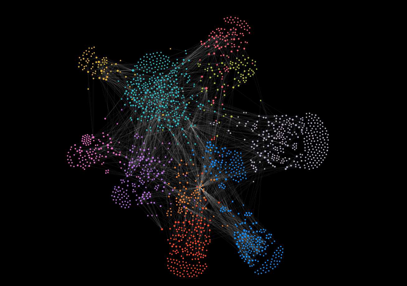
  updatePositions();

We’ve successfully rendered a force-directed graph using PIXI.js! In the next article, I explain in detail the creation of an expandable and collapsible feature for the graph to show or hide subgraphs.